Chapter
Chapter 2: System Model Representation
What is covered
Week 3 12 Oct to 18 Oct 2026
- From physics to model: differential-equation models and system order
- Transfer function representation: from ODE to G(s)
- Poles, zeros and DC gain; stability from pole location
Week 4 19 Oct to 25 Oct 2026
- State-space representation: state variables and the A, B, C, D matrices
- Conversion between ODE, state space and transfer function
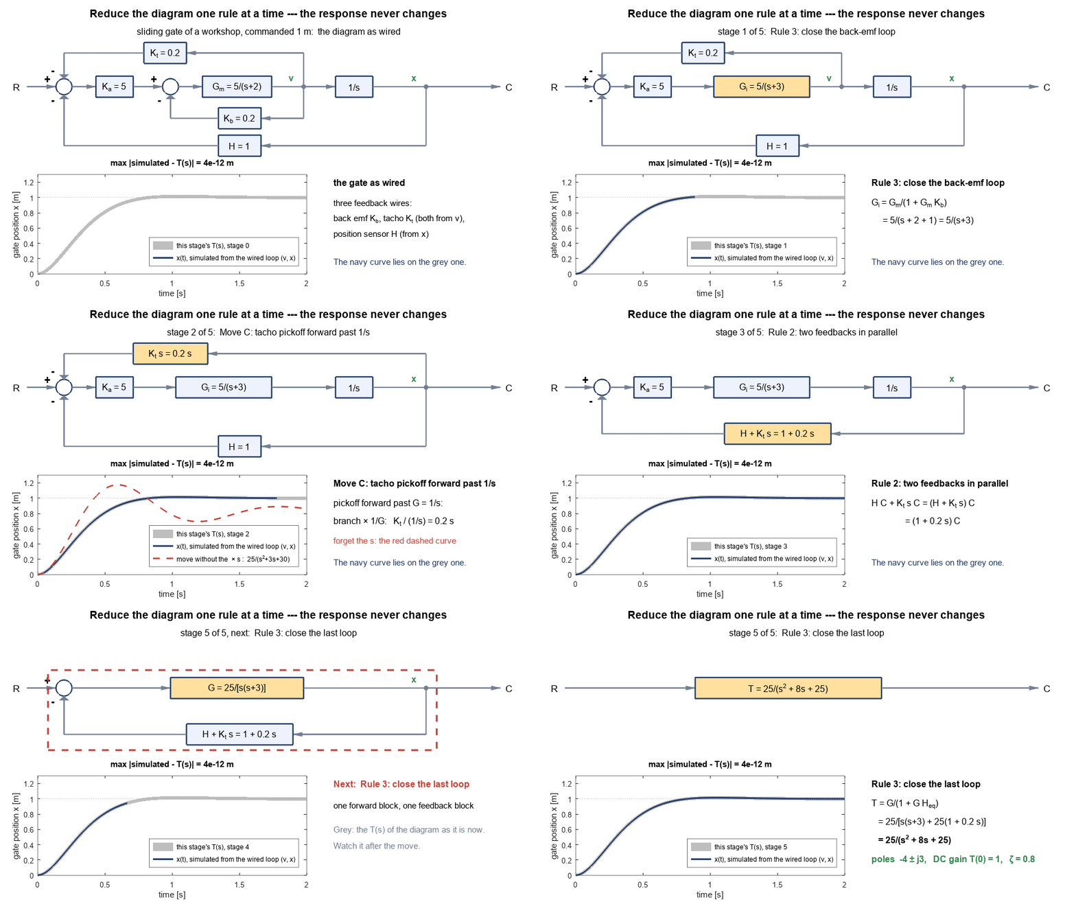
- Block diagram manipulation: cascade, parallel and feedback; moving summing junctions and pick-off points
Week 5 26 Oct to 1 Nov 2026
- Block diagram reduction: worked multi-loop examples
- Signal flow graph and Mason's gain formula
- Chapter 2 review and Q&A
Try it
Cheat sheet
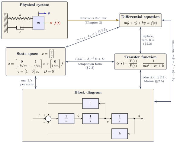 One page for Chapter 2The key picture, which formula to use when, and the ways to lose marksOpen the Chapter 2 cheat sheet
Animations
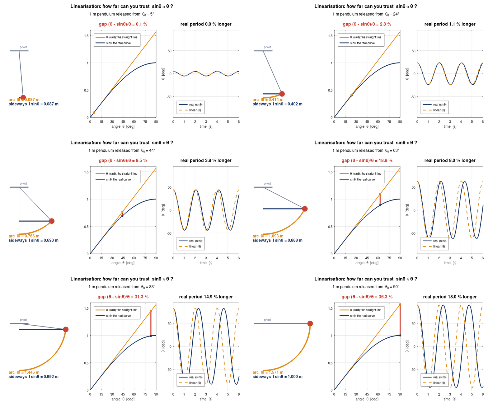
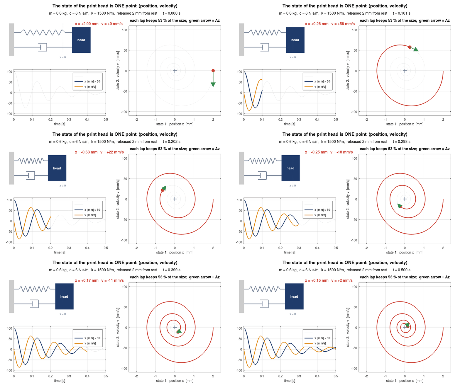
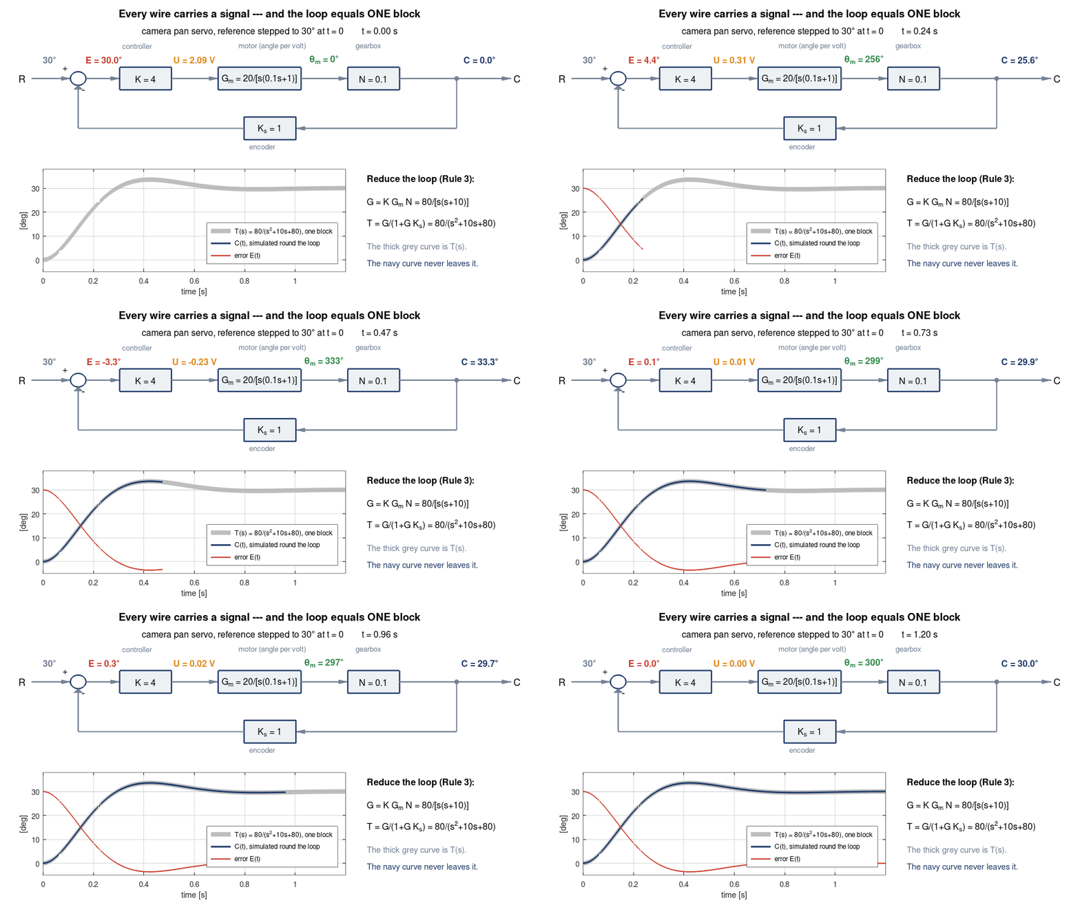
Show the 4 animations from the lecture slides and the chapter overview
Download
- Lecture slides (handout) PDF, 6.6 MB